
By Jark <http://mandelbrot.dazibao.free.fr>
These simple principles are not sufficient to allow generating fancy true-colours pictures... The Sponge of Sierpinsky picture shown here was generated with a heavy raytracing technique, which is out of scope here.
As a matter of fact, the Julia sets and the Mandelbrot Set are the fractals that are at the same time simple enough to be programmed even with QB, and at the same time complex enough to keep you busy for a couple of months.
These two fractals are based on similar iterative formulas (iterative is the master word here...).
Both of them are computed via complex numbers. Complex numbers are, to make it simple, 2D numbers. That means we speak about a double number "z", z being equal to "x+i*y", with i^2=-1. Of course, the computer cannot understand i^2= -1, but it can perfectly understand z1+z2 = (x1+x2) + i * (y1+y2) and z1*z2 = (x1*x2-y1*y2) + i*(x1*y2+x2*y1), and handle complex numbers as a 2D vector (x,y). In other terms, a complex number is a point in the (x,y) plan. For the computer, it is just a pixel...
A Julia set refers to a complex number C=(x0,y0), and is made of all the complex numbers z (i.e the points (x,y) of the plan) for which the suite z(n+1) = z(n) + C does not escape when z(0)= z.
The Mandelbrot Set does not refer to a particular number. It is made of the complex numbers C (C=(x,y) in a plan) for which the suite z(n+1) = z(n) + C does not escape when z(0)= (0,0).
A link between Julia and Mandelbrot ? Well, yes... The M-Set is the set made of the points of the complex plan which has a fully connected Julia Set (i.e. the Julia Set for this (x0,y0) is a plain one-piece object).
Now we can try to prog that:
SCREEN 12
FOR m = 1 TO 640
FOR n = 1 TO 480
p = (m - 320) / 140
q = (n - 240) / 140
x = 0
y = 0
FOR i = 1 TO 90
u = x * x - y * y + p
v = 2 * x * y + q
IF u * u + v * v > 4 THEN GOTO E
x = u
y = v
NEXT i
PSET (m, n), 1
E:
NEXT n
NEXT m
This little prog demonstrates how accessible the Mandelbrot Set can be: 256 bytes of code, and you get your first picture of the most famous fractal!
Now, what you probably want is something that looks "professional". There's no escape: switch directly to true colour pictures! I hear you say: "Hey, that requires complex VESA stuff, or an external lib such as Future Lib". No way, the most reliable technique is to generate a true colour bitmap file... This bitmap will behave as a virtual screen, and it will be fully independent from the hardware.
First, you create a blank bitmap. That routine is equivalent to activating a video mode, and you can specify the desired picture size:
DIM SHARED ScrWidth as Integer
DIM SHARED ScrHeight as Integer
DIM SHARED SaveDir$
DIM SHARED FileNumber%
SUB OpenBmp (Name$, PicWidth, PicHeight)
ScrWidth = PicWidth : ScrHeight = PicHeight
' Bitmap structure parameters
Bw& = ScrWidth : Bh& = ScrHeight : Os& = 54
IF (3 * Bw& MOD (4)) <> 0 THEN PadBytes% = 4 - ((3 * Bw&) MOD (4))
Fs& = (3 * Bw& + PadBytes%) * Bh& + Os&
Ps& = (3 * Bw& + PadBytes%) * Bh&

' Create a binary file
Pic$ = SaveDir$ + Name$ + ".bmp"
FileNumber% = FREEFILE
OPEN Pic$ FOR BINARY AS FileNumber%

' Write the bitmap header
Buffer$ = "BM"                                     'MS-Windows bitmap
Buffer$ = Buffer$ + MKL$(Fs&)                      'File Size
Buffer$ = Buffer$ + CHR$(0) + CHR$(0)              'Reserved 1
Buffer$ = Buffer$ + CHR$(0) + CHR$(0)              'Reserved 2
Buffer$ = Buffer$ + MKL$(Os&)                      'Offset
Buffer$ = Buffer$ + MKL$(40)                       'File Info size
Buffer$ = Buffer$ + MKL$(Bw&)                      'Pic Width
Buffer$ = Buffer$ + MKL$(Bh&)                      'Pic Height
Buffer$ = Buffer$ + CHR$(1) + CHR$(0)              'Number of planes
Buffer$ = Buffer$ + CHR$(24) + CHR$(0)             'Number of bits per pixel
Buffer$ = Buffer$ + MKL$(0)                        'No compression
Buffer$ = Buffer$ + MKL$(Ps&)                      'Image Size
Buffer$ = Buffer$ + MKL$(0)                        'X Size (pixel/meter)
Buffer$ = Buffer$ + MKL$(0)                        'Y Size (pixel/meter)
Buffer$ = Buffer$ + MKL$(0)                        'Colors used
Buffer$ = Buffer$ + MKL$(0)                        'Important colors
PUT FileNumber%, 1, Buffer$

' Fill the bitmap with blank pixels (three bytes per pixel)
FOR Ny& = 1 TO Bh&
Buffer$ = CHR$(0) + CHR$(0) + CHR$(0)
FOR Nx& = 1 TO Bw&
PUT FileNumber%, , Buffer$
NEXT Nx&
Buffer$ = ""
FOR i% = 1 TO PadBytes%
Buffer$ = Buffer$ + CHR$(0)
NEXT i%
PUT FileNumber%, , Buffer$
NEXT Ny&

END SUB
Then you need to plot an RGB combination at a precise pixel. Remember the pixels in a bitmap file go from left to right and from bottom to top, and that the pixel coordinates start at (0,0):
DIM SHARED Red%, Green%, Blue%

SUB Pset24 (x%, y%)

IF x% < 0 OR x% > ScrWidth - 1 OR y% < 0 OR y% > ScrHeight - 1 THEN EXIT SUB
IF Red% < 0 THEN Red% = 0
IF Green% < 0 THEN Green% = 0
IF Blue% < 0 THEN Blue% = 0
IF Red% > 255 THEN Red% = 255
IF Green% > 255 THEN Green% = 255
IF Blue% > 255 THEN Blue% = 255

xp% = x% + 1: yp% = y% + 1
Col$ = CHR$(Blue%) + CHR$(Green%) + CHR$(Red%)
Bw& = ScrWidth: Bh& = ScrHeight
IF (3 * Bw& MOD (4)) <> 0 THEN PadBytes% = 4 - ((3 * Bw&) MOD (4))
LineLength& = Bw& + Bw& + Bw& + PadBytes%
Offset& = 54 + (ScrHeight - yp%) * LineLength& + xp% + xp% + xp% - 2
PUT FileNumber%, Offset&, Col$

END SUB
When your picture is terminated, don't forget to close the file...
SUB CloseBmp
CLOSE FileNumber%
END SUB
Well, here you are: you can now draw true colour pixel with Quick-Basic, with a reliable technique, that will generate a portable picture format. The huge advantage is that even if your picture takes hours to render, you can launch your program as a background task, without being stuck in front of the screen...
Important recommendation: integrate the HSV colorspace in your programs! Working in true-colours directly in RGB is a pain in the back, while introducing HSV makes it really easy... Read the detailed tutorial at The Mandelbrot Dazibao, you will find everything about HSV there.
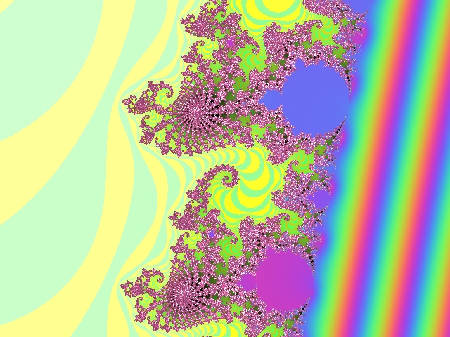
The little program in Screen 12 can now be extrapolated up to a genuine true-colours M-Set Explorer. You will find a 5 steps Mandelbrot Programming Tutorial, written for QB, at The Mandelbrot Dazibao. The main points are:
The following image merges all these techniques:
You can also download and adapt to your taste TC-Mdb which is an interactive, mouse-driven, M-Set explorer written with QB on the basis of the TC-Lib (True-Colour Library for Quick-Basic).
Raytracing is one the most fascinating domains in computer graphics. Merging fractals and 3D techniques can provide a lot of fun and fantastic pictures...
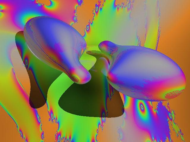
Fractals formulas can be used to generate procedural textures. In the following picture, the background is a cubic shape (x^3+y^3+z^3=0) with a textured Julia set, while the quartic shape is patterned with Mandelbrot sets.
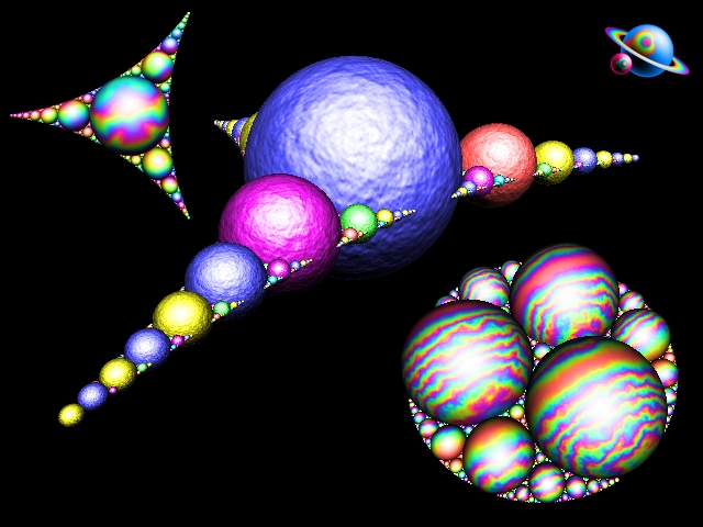
Classical 2D fractals such as the Apollonia fractal can be renewed when you replace the basic circles by raytraced spheres:
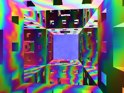
Raytracing also allows plotting regular 3D fractals, like on this zoom inside the Sponge of Sierpinsky:
All the graphics shown in this article were generated with Quick-Basic, with correct results. Yet, QB has some limits, and rendering these complex objects is sometimes really slow. The pleasure of programming with QB is always here, anyway...
If you want to know more about fractals, three sites can be visited:
And of course, The Mandelbrot Dazibao... Think Global, Make Symp'All! ®