Mandelbrot and Julia sets with PANORAMIC and FreeBASIC
By jdebord
I. Introduction
We present here a program written in two BASIC dialects, PANORAMIC and FreeBASIC, to explore the Mandelbrot and Julia sets. These fractal figures are created by iteration of a function of complex variable z → f(z) + c, where c is a complex constant. The present version is limited to the power function f(z) = zp, where p is an integer or real exponent such that p > 1.
The program (sources and executable) are available from the author's web site.
II. The Mandelbrot set
The Mandelbrot set, named after the mathematician Benoît Mandelbrot, corresponds to the case p = 2. More precisely, it is defined as the set of complex numbers c for which the sequence:
z0 = c
zn = (zn-1)2 + c
converges to a finite value.
In practice, the sequence is iterated at each point c in the complex plane. The points belonging to the set are given the same color, and the points outside the set are given a color which depends on their divergence rate.
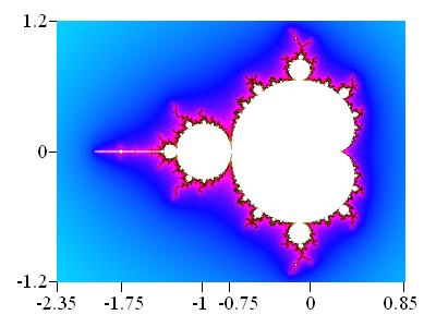
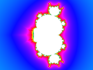
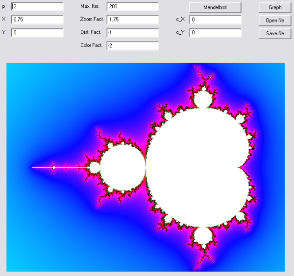
A global view of the Mandelbrot set is shown here:
-
The Mandelbrot set is in white. It is comprised of several parts:
-
a cardioid (heart-shaped curve, at right) which constitutes the main part of the set. The "cusp" of the cardioid is at (0.25, 0)
-
a main disk of radius 0.25 centered at (-1, 0) and tangent to the cardioid at (-0.75, 0)
-
a straight "tip" (leftmost part of the set), showing a mini-Mandelbrot set at the abscissa -1.75
The set is covered with "bulbs" of various sizes emitting filaments. The major bulbs are located at the poles of the cardioid. Each bulb is itself covered with other bulbs, while the filaments give rise to small copies (more or less distorted) of the set. All these structures are repeated at all scales.
Mathematicians have shown that:
-
the Mandelbrot set is included in the circle of radius 2: the complex numbers having a modulus higher than 2 don't belong to the set.
-
the set is connected: all its parts are linked by filaments which can be infinitely thin and therefore not visible on the pictures.
-
-
The immediate vicinity of the set is plotted in dark colors, using the distance estimator method which will be described later.
-
The outside of the set contains the points for which the sequence tends towards infinity. It is colored according to the number of iterations needed to reach a value called the escape radius. When a point gets closer to the set, the number of iterations increases, and it increases faster as the point approaches the set.
III. The Julia sets
These sets, named after the mathematician Gaston Julia, are defined in a manner similar to the Mandelbrot set, except that here the parameter c is constant and the sequence is initialized with the coordinates zpixel of the point:
z0 = zpixel
zn = (zn-1)2 + c
So, there is a Julia set for each value of the parameter c.
It has been shown that:
-
When the point c belongs to the Mandelbrot set, the Julia set is connected, i. e. as a whole.
-
Otherwise, the Julia set is made of an infinity of similar parts.
|
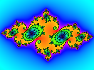
c = (-0.75 , 0) This point belongs to the Mandelbrot set. |
c = (-0.75 , 0.1) This point is outside the Mandelbrot set. The Julia set is disconnected. |
 |
 |
IV. Variation of the exponent p
IV.A. Integer exponent
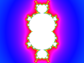
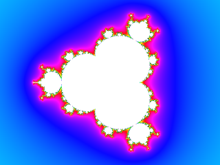
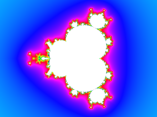
For the integer values of p (> 2) the Mandelbrot set is centered at (0,0) and is comprised of (p - 1) symmetrical lobes. When p is even, one of these lobes is located along the negative Ox axis. There is no such lobe when p is odd.
|
p = 3 2 lobes (symmetry of order 2). No lobe on the Ox axis. |
p = 4 3 lobes (symmetry of order 3). One lobe on the Ox axis. |
 |
 |
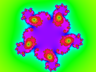
The corresponding Julia sets have a symmetry of order p.
Example with p = 5 and c = (-0.5 , 0.64) :
 |
IV.B. Non-integer exponent
The pictures display discontinuities. This is due to the fact that, for non-integer values of p, zp is evaluated as exp(p ln z). But the logarithm of a complex number is a multi-valued function. The discontinuities arise from the choice of a single value at each point.
Example with p = 3.5 :
 |
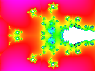
It is interesting to study the transition from an odd integer p to an even integer while following the intermediaite values. We can observe the progressive formation of the lobe located along the Ox axis. This lobe is formed by fusion of multiple "buds" which develop progressively and are surrounded by complex structures.
|
p = 3.85 A step of the formation of the lobe located on the Ox axis, from several fragments. |
p = 3.85 Zoom (× 10) of the previous image, showing some fragments and the structures around them. |
 |
 |
V. Theoretical aspects
We will explain here some mathematical principles involved in the computation of these sets. An elementary knowledge of complex numbers is required.
V.A. Iteration of the complex function
The sequence zn = (zn-1)p + c is iterated until the modulus |zn| exceeds the escape radius, or the iteration number n exceeds a predefined value. In the last case, the point is considered as belonging to the Mandelbrot set.
V.B. The distance estimator
As its name implies, this parameter estimates the distance between the tested point and the Mandelbrot set. It is computed by using the fact that the iteration number required to reach the escape radius increases faster as the point approaches the set. This rate is estimated by the derivative of the iterated function.
z'n = p (zn-1)p-1 (z'n-1) + 1
with z'0 = 0
z'n = p (zn-1)p-1 (z'n-1)
with z'0 = 1
-
For the Mandelbrot set, the function depends on the parameter c. We must then derive with respect to this parameter:
-
For the Julia set, the parameter c is constant. The derivative reduces to:
At the end of the iterations, the distance estimator is given by:
D = ( p |zn| ln |zn| ) / |z'n|
The weaker this value, the closer we are to the set.
V.C. The continuous dwell method
As we have shown previously, points outside the Mandelbrot set are colored according to the iteration number required to reach the escape radius. At the vicinity of the set, this number varies rapidly from one point to another, resulting in a color mixing which makes the picture look "fuzzy". To avoid this effect, it is possible to "smooth" the variation of iteration numbers by means of a logarithmic transform. The formula used here is the following:
Dwell = n - logp ( ln |zn| ) + logp ( ln Esc )
where Esc denotes the escape radius. The function logp is the base-p logarithm, such that logp z = ln z / ln p
VI. The FBMANDEL DLL
The above computations are implemented in the fbmandel.bas DLL, written in FreeBASIC and based on the fbcomplex library for complex numbers. We present here the main algorithms used by the DLL, as well as the exported functions.
VI.A. Picture format
The picture is 640 × 480, 32 bits. It is centered at (x0 , y0). The zoom is defined by the ZoomFact parameter, such that the value ZoomFact = 1 corresponds to a vertical scale of 4, resulting in a horizontal scale of 4 × (640 / 480) = 5,333 ... The vertical scale for a given ZoomFact value is therefore 4 / ZoomFact. If Scale denotes the pixel scale, we can define a scale factor:
ScaleFact = 4 / (Scale * ZoomFact)
This factor represents the distance between 2 pixels. So, the pixel coordinates (Nx, Ny) of a point are converted to the algebraic coordinates (x, y) by:
   x = x0 + ScaleFact * (Nx - HalfPicWidth)
   y = y0 - ScaleFact * (Ny - HalfPicHeight)
where HalfPicWidth and HalfPicHeight denote the half-width and half-height of the picture, i. e. 320 and 240 in our case.
A complete scan of the picture is performed with two loops:
  for Ny = 0 to PicHeight - 1
     yt = y0 - ScaleFact * (Ny - HalfPicHeight)
     for Nx = 0 to PicWidth - 1
       xt = x0 + ScaleFact * (Nx - HalfPicWidth)
           pset (Nx, Ny), Mandelbrot(xt, yt)
     next Nx
   next Ny
where PicWidth and PicHeight denote the width and height of the picture, i. e. 640 and 480 in our case. The Mandelbrot function returns the color of the point.
VI.B. Computing the iterations
The Mandelbrot function performs the iterations at the point of algebraic coordinates (xt, yt) by computing simultaneously the complex function zn and its derivative z'n, according to the following code:
  if Julia then
     c = cJulia
     z = Cmplx(xt, yt)
     dz = C_one
   else
     c = Cmplx(xt, yt)
     z = C_zero
     dz = C_zero
   end if
   Iter = 0
   Module = CAbs(z)
   do while Iter < MaxIter and Module < Esc
     zp1 = z ^ p1
     zn = z * zp1 + c
     dzn = p * zp1 * dz
     if not Julia then dzn = dzn + 1
     Module = CAbs(zn)
     z = zn
     dz = dzn
     Iter = Iter + 1
   loop
where:
- Julia indicates if we are computing a Julia set
- cJulia corresponds to the parameter c for the Julia set
- C_zero and C_one are the complex constants (0,0) and (1,0)
- the function Cmplx(x, y) returns the complex number (x, y)
- the function CAbs returns the modulus of a complex number
- p1 = p - 1
The iterations can be terminated in two ways:
-
If the iteration number reaches MaxIter, the point is considered as belonging to the Mandelbrot set, and plotted in white:
if Iter = MaxIter then return &HFFFFFF
This method does not ensure that the sequence converges since rigorously we should perform an infinite number of iterations! We take the risk to include in the set some points located very closely to its frontier. This will result a "fuzzy" aspect on the graphic. In this case, the solution is to increase MaxIter, at the expense of the computation time. -
If the modulus of the complex number reaches the value of the escape radius, the sequence diverges and the point does not belong to the set. In this case, we compute the distance estimator and the continuous dwell :
  LnMod = log(Module)
   Dist = p * Module * LnMod / CAbs(dzn)
   Dwell = Iter - log(LnMod) / Lnp + LLE
where Lnp denotes the natural logarithm of p and LLE = logp ( ln Esc )
The value of the escape radius has been fixed at 1010. It is the distance estimator algorithm which needs such a high value.
VI.C. Color attribution
We use a simplified version of an algorithm described by Robert Munafo. Its main features are the following:
-
The colors are defined in the HSV (Hue, Saturation, Value) space.
-
The value is attributed according to the distance estimator, so that the points close to the set appear in dark shades. This facilitates the detection of the tiniest parts of the set, which may not be visible at a given zooming.
-
The hue and the saturation are attributed according to the continuous dwell.
VI.D. Functions exported by the DLL
The DLL exports 4 functions:
- SetFractal
This function initialises the exponent p and the coordinates c_X et c_Y of the parameter c for the Julia set. If these coordinates are both null, the Mandelbrot set will be plotted.
Example call from PANORAMIC:
  dim i%, p, c_X, c_Y

  p = 2
  c_X = -0.75
  c_Y = 0.1
  i% = dll_call3("SetFractal", adr(p), adr(c_X), adr(c_Y))
The function returns 0 if p > 1, -1 otherwise.
- SetGraphParams
This function defines the graphic parameters:
- x0, y0 : coordinates of the picture center
- MaxIter : maximal number of iterations
- ZoomFact : zoom factor (max. 1014)
- DistFact : coloration factor according to the distance estimator method (see Notes below)
- ColorFact : factor controlling the color range
Notes :
-
The luminosity is controlled by the parameter DistFact and increases with it.
-
The color density is controlled by the parameter ColorFact : the higher this parameter (in absolute value), the more colors on the picture. For a black and white image, set ColorFact to zero.
-
If ColorFact is positive, the alternance of color stripes around the set is enhanced by darkening every other stripe. This effect may be suppressed by giving a negative value to ColorFact : in this case, the coloring will look more like a continuous gradient (as with the pictures displayed in the present article).
Example call from PANORAMIC:
dim i%, x0, y0, MaxIter%, ZoomFact, DistFact, ColorFact x0 = -0.75 y0 = 0 MaxIter% = 100 ZoomFact = 1.5 DistFact = -1 ColorFact = 1 i% = dll_call6("SetGraphParams", adr(x0), adr(y0), MaxIter%, adr(ZoomFact), adr(DistFact), adr(ColorFact)) - MandelGraph
This function plots the set. It has no parameters and always returns zero. It must be called after the two previous functions.
Example call from PANORAMIC:
i% = dll_call0("MandelGraph") - GetCoord
This function computes the algebraic coordinates (x, y) of a point, knowing its pixel coordinates (Nx, Ny) and the algebraic coordinates (x0, y0) of the center.
Example call from PANORAMIC:
  dim i%, Nx%, Ny%, x0, y0, x, y
  x0 = -0.75
  y0 = 0.15

  Nx% = 200
  Ny% = 100
  i% = dll_call6("GetCoord", adr(x0), adr(y0), Nx%, Ny%, adr(x), adr(y))
This function must be used after a call to SetGraphParams otherwise the scale factor would not be initialised.
VII. The PANOMAND program
This program written in PANORAMIC supplies a graphic interface to the previous DLL.
The values of the various parameters are entered in the corresponding cells. The X and Y coordinates relate to the center of the picture. The "Graph" button starts the computation. The picture is plotted in a secondary window, then transferred to the main window. The picture is saved in the file fractal.bmp. The parameters are saved in the text file fractal.par. The "Save file" button allows to save to another file name, while the "Open file" button allows to load a previously saved picture.
To switch from the Mandelbrot set to the Julia set, click on the "Mandelbrot" button. Its caption will become "Julia" and the coordinates of the current Mandelbrot picture will become the c parameter of the Julia set, appearing in the "c_X" and "c_Y" boxes. The old coordinates will become zero, to ensure that the Julia set is centered at (0, 0).
By clicking on a point of the picture, we get its coordinates in the cells X and Y. We can then zoom on the selected point by increasing the zoom factor.
VIII. Conclusion
We hope that this program will incite you to further explore the Mandelbrot and Julia sets.
Don't hesitate to generate your own pictures. There are still plenty of things to discover!
As an example, the author's web site displays an exploration of the seahorse valley, located between the cardioid and the main circle. Note that the web site is in french, but the example consists mainly of pictures, so that you can enjoy them even if you can't read french!
IX. Links
-
Mandelbrot Dazibao. Excellent site with tutorials and QBasic programs. PANOMAND is based on one of them.
-
Mu-Ency. Encyclopedia of Mandelbrot set, by Robert Munafo. Describes the coloring method used in PANOMAND.
-
High Precision Deep Zoom. Images of Mandelbrot set and related fractals at very high zooms.
-
Fractal forums. An impressive collection of forums covering all aspects of fractals.